Divide and Conquer, Sorting and Searching, and Randomized Algorithms

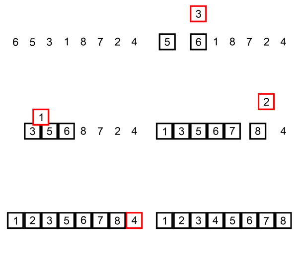
Insertion Sort

Insertion Sort: Pseudocode

 1
 2
 3
 4
 5
 6
 7
 8
 9
10

INSERTION-SORT(A)

for j = 2 to A.length
	key = A[j]
	// Insert A[j] into the sorted sequence A[1..j-1].
	i = j - 1
	while i > 0 and A[j] > key
		A[i+1] = A[i]
		i = i - 1
	A[i + 1] = key

Insertion Sort: Complexity analysis

insertion sort has a best-case running time of $$\theta{(n)}$$ (pronounced “theta of n”).

insertion sort has an average and worst-case running time of $$\theta{(n^2)}$$ (pronounced “theta of n-squared”).

Insertion Sort: Advantages

Efficient for (quite) small data sets

Stable; i.e., does not change the relative order of elements with equal keys

In-place; i.e., only requires a constant amount O(1) of additional memory space

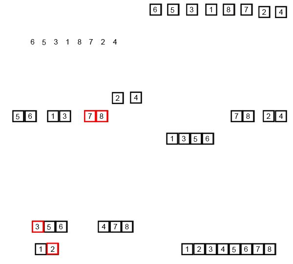
Merge Sort

Merge Sort: Pseudocode

 1
 2
 3
 4
 5
 6
 7
 8
 9
10
11
12
13
14
15
16
17
18
19
20

MERGE(A; p, q, r)

n1 = q - p + 1
n2 = r - q
let L[1 ... n1 + 1] and R[1 ... n2 + 1] be new arrays
for i = 1 to n1
	L[i] = A[p + i - 1]
for j = 1 to n2
	R[j] = A[q+j]
L[n1 + 1] = INF
R[n2 + 1] = INF
i = 1
j = 1
for k = p to r
	if L[i] <= R[j]
		A[k] = L[i]
		i = i + 1
	else
		A[k] = R[j]
		j = j + 1

1
2
3
4
5
6
7

MERGE-SORT(A, p, r)

if p < r
	q = (p +r) / 2
	MERGE-SORT(A, p, q)
	MERGE-SORT(A, q+1, r)
	MERGE(A, p, q, r)

Merge Sort: Complexity analysis

merge sort has an average and worst-case running time of $\theta(n \lg n)$

merge sort’s worst-case space complexity $\theta(n)$

Merge Sort: Advantages

Merge sort is more efficient than quicksort for some types of lists if the data to be sorted can only be efficiently accessed sequentially.

Unlike some (efficient) implementations of quicksort, merge sort is a stable sort.

Merge sort is often the best choice for sorting a linked list: in this situation it is relatively easy to implement a merge sort in such a way that it requires only $\theta(1)$ extra space, and the slow random-access performance of a linked list makes some other algorithms (such as quicksort) perform poorly, and others (such as heapsort) completely impossible.

Bubble Sort

Bubble Sort: Pseudocode

1
2
3
4
5

BUBBLESORT(A)
for i = 1 to A.length - 1
	for j D A:length downto i C 1
		if A[j]  < A[j - 1]
			exchange A[j] with A[j - 1]

Bubble Sort: Complexity analysis

Bubble sort has a worst-case and average complexity of $O(n^2)$

Quicksort

Quicksort: Pseudocode

1
2
3
4
5

QUICKSORT(A, p, r)
if p < r
	q = PARTITION(A, p, r)
	QUICKSORT(A, p, q - 1)
	QUICKSORT(A, q + 1, r)

1
2
3
4
5
6
7
8
9

PARTITION(A, p, r)
x = A[r]
i = p - 1
for j = p to r - 1
	if A[j] <= x
		i = i + 1
		exchange A[i] with A[j]
exchange A[i + 1] with A[r]
return i + 1

Quicksort: Complexity analysis

The quicksort algorithm has a worst-case running time of $\theta(n^2)$.

Despite this slow worst-case running time, quicksort is often the best practical choice for sorting because it is remarkably efficient on the average: its expected running time is $\theta(n \lg n)$.

The running time of quicksort depends on whether the partitioning is balanced or unbalanced, which in turn depends on which elements are used for partitioning. If the partitioning is balanced, the algorithm runs asymptotically as fast as merge sort. If the partitioning is unbalanced, however, it can run asymptotically as slowly as insertion sort.

The average-case running time of quicksort is much closer to the best case than to the worst case.

In fact, any split of constant proportionality yields a recursion tree of depth $\theta(n \lg n)$, where the cost at each level is $O(n)$. The running time is therefore $\theta(n \lg n)$ whenever the split has constant proportionality.

Quicksort: Scenses

It has the advantage of sorting in place.

Moreover, the $\theta(n^2)$ running time occurs when the input array is already completely sorted—a common situation in which insertion sort runs in $O(n)$ time.

A randomized version of quicksort

Randomized quicksort: Pseudocode

1
2
3
4

RANDOMIZED-PARTITION(A, p, r)
i = RANDOM(p, r)
exchange A[r] with A[i]
return PARTITION(A, p, r)

1
2
3
4
5

RANDOMIZED-QUICKSORT(A, p, r)
if p < r
	q = RANDOMIZED-PARTITION(A, p, r)
	RANDOMIZED-QUICKSORT(A, p, q - 1)
	RANDOMIZED-QUICKSORT(A, q + 1, r)

Randomized quicksort: Complexity analysis

the (worst-case) running time of quicksort is $\theta(n^2)$.

the expected running time of RANDOMIZED -QUICKSORT is $O(n \lg n)$.

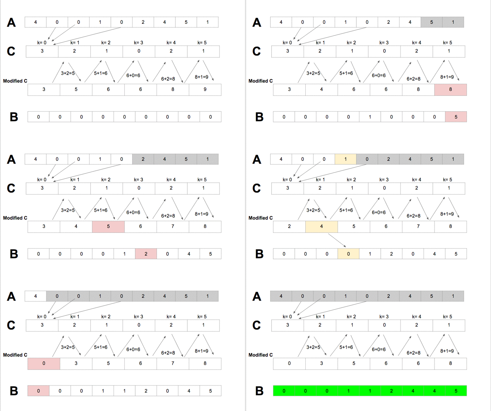
Counting Sort

Counting Sort: Pseudocode

 1
 2
 3
 4
 5
 6
 7
 8
 9
10
11
12
13
14

COUNTING-SORT(A, B, k)

let C[0 ... k] be a new array
for i = 0 to k
	C[i] = 0
for j = 1 to A.length
	C[A[j]] = C[A[j]] + 1
// C[i] now contains the number of elements equal to i.
for i = 1 to k
	C[i] = C[i] + C[i - 1]
// C[i] now contains the number of elements less than or equal to i.
for j = A.length downto 1
	B[C[A[j]]] = A[j]
	C[A[j]] = C[A[j]] - 1

Counting Sort: Complexity analysis

Counting sort has time complexity of $O(k + n)$

Because it uses arrays of length $k + 1$ and $n$, the total space usage of the algorithm is also $O(n + k)$.

Counting Sort: Scenes

it is an integer sorting algorithm

it is a stable sort.

Radix Sort

Radix Sort: Pseudocode

1
2
3
4

RADIX-SORT(A, d)

for i = 1 to d
	use a stable sort to sort array A on digit i

Radix Sort: Complexity analysis

Radix sort operates in $O(nw)$ time, where $n$ is the number of keys, and $w$ is the key length.

Radix Sort: Scenes

Moreover, the version of radix sort that uses counting sort as the intermediate stable sort does not sort in place, which many of the ‚.n lg n/-time comparison sorts do. Thus, when primary memory storage is at a premium, we might prefer an in-place algorithm such as quicksort.

Bucket Sort

Bucket Sort: Pseudocode

 1
 2
 3
 4
 5
 6
 7
 8
 9
10
11

BUCKET-SORT(A)

let B[0 ... n - 1] be a new array
n = A.length
for i = 0 to n - 1
	make B[i] an empty list
for i = 1 to n
	insert A[i] into list B[n A[i]]
for i = 0 to n - 1
	sort list B[i] with insertion sort
concatenate the lists B[0], B[1], ..., B[n - 1] together in order

Bucket Sort: Complexity analysis

Bucket sort has an average complexity of $\theta(n)$

Bucket sort has a worst-cast complexity of $\theta(n^2)$

Summarizes the sorting algorithms