SQL Tutorial

Lexical elements

Literal Values

String Literals

Numeric Literals

Numeric literals can be represented by simple values.

Date and Time Literals

Characters and date literals must be enclosed within single quotes.

Hexadecimal Literals

Bit-Value Literals

Boolean Literals

NULL Values

Identifiers

Identifiers must start with an alphabetic character.

Keywords and Reserved Words

Reserved words cannot be used as identifiers unless enclosed with double quotes.

Statements may be split across lines, but keywords may not.

Punctuation

• A query normally consists of an SQL statement followed by a semicolon.
• Identifiers, operator names, and literals are separated by one or more spaces or other delimiters.
• A comma (,) separates parameters without a clause.
• A space separates a clause.

Comments

Single Line Comments

1
2
3

SELECT * FROM customers; 
-- This is a comment that explains 
   the purpose of the query.

Multi-Line Comments:

1
2
3
4
5

/* multi line comment

another comment */

SELECT * FROM Customers; 

In-Line Comments:

1
2
3
4
5

SELECT customer_name, 
/* This column contains the name of 
the customer / order_date / 
This column contains the date the
order was placed */ FROM orders;

SQL Data Types

SQL Functions

Mathematical Functions

Window Functions

The aggregated values can’t be directly used with non-aggregated values to obtain a result. Thus one can use the following concepts:

1. Using Join

   1 2 3 4 5 6 7 8 9 10

   SELECT ENAME, SAL, EMP.JOB, SUBTABLE.MAXSAL, SUBTABLE.MINSAL, SUBTABLE.AVGSAL, SUBTABLE.SUMSAL FROM EMP INNER JOIN (SELECT JOB, MAX(SAL) MAXSAL, MIN(SAL) MINSAL, AVG(SAL) AVGSAL, SUM(SAL) SUMSAL FROM EMP GROUP BY JOB) SUBTABLE ON EMP.JOB = SUBTABLE.JOB;

   Ename	Sal	Job	MaxSal	MinSal	AvgSal	SumSal
   SCOTT	3300	ANALYST	3300	1925	2841.67	8525
   HENRY	1925	ANALYST	3300	1925	2841.67	8525
   FORD	3300	ANALYST	3300	1925	2841.67	8525
   SMITH	3300	CLERK	3300	1045	1746.25	6985
   MILLER	1430	CLERK	3300	1045	1746.25	6985

2. Using Over clause

To use a window function (or treat an aggregate function as a window function), include an OVER clause following the function call. The OVER clause has two forms:

1
2

over_clause:
    {OVER (window_spec) | OVER window_name}

• In the first case, the window specification appears directly in the OVER clause, between the parentheses.
• In the second case, window_name is the name for a window specification defined by a WINDOW clause elsewhere in the query.

1
2

window_spec:
    [window_name] [partition_clause] [order_clause] [frame_clause]

If OVER() is empty, the window consists of all query rows and the window function computes a result using all rows. Otherwise, the clauses present within the parentheses determine which query rows are used to compute the function result and how they are partitioned and ordered

• window_name: The name of a window defined by a WINDOW clause elsewhere in the query. If window_name appears by itself within the OVER clause, it completely defines the window. If partitioning, ordering, or framing clauses are also given, they modify interpretation of the named window.

• partition_clause: A PARTITION BY clause indicates how to divide the query rows into groups. The window function result for a given row is based on the rows of the partition that contains the row. If PARTITION BY is omitted, there is a single partition consisting of all query rows.

  partition_clause has this syntax:

  1 2	partition_clause: PARTITION BY expr [, expr] ...

  OVER CLAUSE along with PARTITION BY is used to break up data into partitions.

  The specified function operates for each partiton.

• order_clause: An ORDER BY clause indicates how to sort rows in each partition.

  order_clause has this syntax:

  1 2	order_clause: ORDER BY expr [ASC|DESC] [, expr [ASC|DESC]] ...

• frame_clause: A frame is a subset of the current partition and the frame clause specifies how to define the subset.

The farmers share their production data, which is stored in the orange_production table you see below :

For example, if our farmers want to have a report of every farmer record alongside the total of orange production in 2017, we’d write this query:

1
2
3
4
5

SELECT farmer_name,
       kilos_produced,
       SUM(kilos_produced) OVER() total_produced
 FROM  orange_production
WHERE  crop_year = 2017

Here, the OVER clause constructs a window that includes all the records returned by the query – in other words, all the records for year 2017. The result is:

Let’s look at an example of a sliding window. Suppose our farmers want to see their own production along with the total production of the same orange variety.

1
2
3
4
5
6

SELECT farmer_name,
       orange_variety,
     crop_year,
       kilos_produced,
       SUM(kilos_produced) OVER(PARTITION BY orange_variety) AS total_same_variety
FROM orange_production

The clause OVER(PARTITION BY orange_variety) creates windows by grouping all the records with the same value in the orange_variety column. This gives us two windows: ‘Golden’ and ‘SuperSun’.

Now you can see the result of the query:

Perhaps each farmer prefers to compare his production against the total production for the same variety in the same year. To do that, we need to add the column crop_year to the PARTITION BY clause. The query will be as follows:

1
2
3
4
5
6

SELECT farmer,
       orange_variety,
     crop_year,
       kilos_produced,
       SUM(kilos_produced) OVER(PARTITION BY orange_variety, crop_year)                                                                                                                    AS total_same_variety_year
   FROM orange_production

The clause OVER(PARTITION BY orange_variety, crop_year) creates windows by grouping all records with the same value in the orange_variety and crop_year columns.

And the query results are:

First up, we’ll use the sub-clause ORDER BY in the OVER clause. ORDER BY will generate a window with the records ordered by a defined criteria. Some functions (like SUM(), LAG(), LEAD(), and NTH_VALUE()) can return different results depending on the order of the rows inside the window. Let’s suppose that Farmer Pierre wants to know his cumulative production over the years:

1
2
3
4
5
6

SELECT farmer,
       crop_year,
       kilos_produced,
       SUM(kilos_produced) OVER(ORDER BY crop_year) cumulative_previous_years
 FROM  orange_production
WHERE  farmer = ‘Pierre’

We can see the result of this cumulative SUM() in the result table:

Suppose the farmers want a report showing the total produced by each farmer every year and the total of the previous years. Then we need to partition by the farmer column and order by crop_year:

1
2
3
4
5

SELECT farmer,
       crop_year,
       kilos_produced,
       SUM(kilos_produced) OVER(PARTITION BY farmer ORDER BY crop_year) cumulative_kilos_produced
   FROM orange_production

You can see this in the results table:

SQL Operators

Arithmetic operator

Comparison operator

Logical operator

Operators with Subqueries

LIKE Operator

LIKE is a string comparison operator.

With LIKE you can use the following two wildcard characters in the pattern:

• % matches any number of characters, even zero characters.

• _ matches exactly one character.

• % matches one % character.

• \_ matches one _ character.

One important thing to note about the LIKE operator is that it is case-insensitive by default in most database systems. This means that if you search for “apple” using the LIKE operator, it will return results that include “Apple”, “APPLE”, “aPpLe”, and so on.

For making the LIKE operator case-sensitive, you can use the “BINARY” keyword in MySQL or the “COLLATE” keyword in other database systems.

1

SELECT * FROM products WHERE name LIKE BINARY 'apple%'

Concatenation Operator

|| or concatenation operator is use to link columns or character strings.

1

SELECT first_name, last_name, first_name || last_name FROM table_name;

MINUS Operator

The Minus Operator in SQL is used with two SELECT statements.

MINUS operator will return only those rows which are unique in only first SELECT query and not those rows which are common to both first and second SELECT queries.

 1
 2
 3
 4
 5
 6
 7
 8
 9
10
11

SELECT 
	column1 , column2 , ... columnN
FROM 
	table_name
WHERE condition
MINUS
SELECT 
	column1 , column2 , ... columnN
FROM 
	table_name
WHERE condition;

SQL Statements

Data definition language (DDL)

CREATE Statement

This command is used to create the database or its objects (like table, index, function, views, store procedure, and triggers).

CREATE TABLE Statement

1

CREATE TABLE [table name] ( [column definitions] ) [table parameters]

Constraints

Constraints can be specified when the table is created with the CREATE TABLE statement, or after the table is created with the ALTER TABLE statement.

1
2
3
4
5
6

CREATE TABLE table_name (
    column1 datatype constraint,
    column2 datatype constraint,
    column3 datatype constraint,
    ....
);

The available constraints in SQL are:

• NOT NULL
• UNIQUE
• PRIMARY KEY: A combination of a NOT NULL and UNIQUE. Uniquely identifies each row in a table. A primary key constraint depicts a key comprising one or more columns. Only one primary key per table exist although Primary key may have multiple columns.
• FOREIGN KEY
• CHECK: Ensures that the values in a column satisfies a specific condition
• DEFAULT: Sets a default value for a column if no value is specified

SQL PRIMARY KEY at Column Level :

1
2
3
4
5

Create Table person (
    id int NOT NULL PRIMARY KEY, 
    name varchar2(20), 
    address varchar2(50)
);

You don’t need to specify NOT NULL for primary key columns, they are set automatically to NOT NULL.

SQL PRIMARY KEY at Table Level :

1
2
3
4
5
6

Create Table person (
    id int NOT NULL, 
    name varchar2(20), 
    address varchar2(50),
    PRIMARY KEY(id, name)
);

Here, you have only one Primary Key in a table but it consists of Multiple Columns(Id, Name).

 1
 2
 3
 4
 5
 6
 7
 8
 9
10
11
12
13
14
15
16
17
18
19
20
21
22
23
24
25
26
27
28

CREATE TABLE product (
    category INT NOT NULL, id INT NOT NULL,
    price DECIMAL,
    PRIMARY KEY(category, id)
);

CREATE TABLE customer (
    id INT NOT NULL,
    PRIMARY KEY (id)
);

CREATE TABLE product_order (
    no INT NOT NULL AUTO_INCREMENT,
    product_category INT NOT NULL,
    product_id INT NOT NULL,
    customer_id INT NOT NULL,

    PRIMARY KEY(no),
    INDEX (product_category, product_id),
    INDEX (customer_id),

    FOREIGN KEY (product_category, product_id)
      REFERENCES product(category, id)
      ON UPDATE CASCADE ON DELETE RESTRICT,

    FOREIGN KEY (customer_id)
      REFERENCES customer(id)
);

1
2
3
4
5
6
7
8
9

CREATE TABLE t1
(
  CHECK (c1 <> c2),
  c1 INT CHECK (c1 > 10),
  c2 INT CONSTRAINT c2_positive CHECK (c2 > 0),
  c3 INT CHECK (c3 < 100),
  CONSTRAINT c1_nonzero CHECK (c1 <> 0),
  CHECK (c1 > c3)
);

• The first constraint is a table constraint: It occurs outside any column definition, so it can (and does) refer to multiple table columns. This constraint contains forward references to columns not defined yet. No constraint name is specified, so RDBMS generates a name.
• The next three constraints are column constraints: Each occurs within a column definition, and thus can refer only to the column being defined. One of the constraints is named explicitly. RDBMS generates a name for each of the other two.
• The last two constraints are table constraints. One of them is named explicitly. RDBMS generates a name for the other one.
• The SQL standard specifies that all types of constraints (primary key, unique index, foreign key, check) belong to the same namespace. In MySQL, each constraint type has its own namespace per schema (database). Consequently, CHECK constraint names must be unique per schema.
• Beginning generated constraint names with the table name helps ensure schema uniqueness because table names also must be unique within the schema.

FOREIGN KEY Constraints

Foreign keys permit cross-referencing related data across tables, and foreign key constraints help keep the related data consistent.

The essential syntax for a defining a foreign key constraint in a CREATE TABLE or ALTER TABLE statement includes the following:

1
2
3
4
5
6
7
8

[CONSTRAINT [symbol]] FOREIGN KEY
    [index_name] (col_name, ...)
    REFERENCES tbl_name (col_name,...)
    [ON DELETE reference_option]
    [ON UPDATE reference_option]

reference_option:
    RESTRICT | CASCADE | SET NULL | NO ACTION | SET DEFAULT

Referential Actions:

• CASCADE: Delete or update the row from the parent table and automatically delete or update the matching rows in the child table. (级联)
• SET NULL: Delete or update the row from the parent table and set the foreign key column or columns in the child table to NULL.
• RESTRICT: Rejects the delete or update operation for the parent table. Specifying RESTRICT (or NO ACTION) is the same as omitting the ON DELETE or ON UPDATE clause.
• NO ACTION: A keyword from standard SQL. For InnoDB, this is equivalent to RESTRICT; the delete or update operation for the parent table is immediately rejected if there is a related foreign key value in the referenced table.
• SET DEFAULT: This action is recognized by the MySQL parser, but both InnoDB and NDB reject table definitions containing ON DELETE SET DEFAULT or ON UPDATE SET DEFAULT clauses.

 1
 2
 3
 4
 5
 6
 7
 8
 9
10
11
12
13

CREATE TABLE parent (
    id INT NOT NULL,
    PRIMARY KEY (id)
);

CREATE TABLE child (
    id INT,
    parent_id INT,
    INDEX par_ind (parent_id),
    FOREIGN KEY (parent_id)
        REFERENCES parent(id)
        ON DELETE CASCADE
);

1

ALTER TABLE table_name DROP FOREIGN KEY foreign_key_name;

CHECK Constraints

1

CHECK (expr)

Files Created by CREATE TABLE CREATE TEMPORARY TABLE Statement CREATE TABLE … LIKE Statement

CREATE TABLE … SELECT Statement

You can create one table from another by adding a SELECT statement at the end of the CREATE TABLE statement:

1

CREATE TABLE new_table_name [AS] SELECT * FROM existing_table_name;

FOREIGN KEY Constraints CHECK Constraints Silent Column Specification Changes CREATE TABLE and Generated Columns Secondary Indexes and Generated Columns Invisible Columns Generated Invisible Primary Keys Setting NDB Comment Options

CREATE DATABASE Statement CREATE EVENT Statement CREATE FUNCTION Statement CREATE LOGFILE GROUP Statement CREATE PROCEDURE and CREATE FUNCTION Statements CREATE SERVER Statement CREATE SPATIAL REFERENCE SYSTEM Statement CREATE TABLESPACE Statement CREATE TRIGGER Statement

CREATE VIEW Statement

Views in SQL are kind of virtual tables.

1
2
3

CREATE VIEW 
	view_name [(column_list)]
AS select_statement;

To see the data in the View, we can query the view in the same manner as we query a table.

1

SELECT * FROM view_name;

CREATE ROLE Statement

A role is created to ease the setup and maintenance of the security model. It is a named group of related privileges that can be granted to the user.

1

CREATE ROLE [IF NOT EXISTS] role_name [, role_name ];

CREATE INDEX Statement

An index is a schema object. It is used by the server to speed up the retrieval of rows by using a pointer. It can reduce disk I/O(input/output) by using a rapid path access method to locate data quickly.

An index helps to speed up select queries and where clauses, but it slows down data input, with the update and the insert statements.

1

CREATE [UNIQUE | FULLTEXT | SPATIAL] INDEX index_name ON table_name col_name;

When Should Indexes be Created?

• A column contains a wide range of values.
• A column does not contain a large number of null values.
• One or more columns are frequently used together in a where clause or a join condition.

When Should Indexes be Avoided?

• The table is small
• The columns are not often used as a condition in the query
• The column is updated frequently

When executing a query on a table having huge data ( > 100000 rows ), MySQL performs a full table scan which takes much time and the server usually gets timed out. To avoid this always check the explain option for the query within MySQL which tells us about the state of execution. It shows which columns are being used and whether it will be a threat to huge data. On basis of the columns repeated in a similar order in condition.

We should also be careful to not make an index for each query as creating indexes also take storage and when the amount of data is huge it will create a problem. In general, it’s a good practice to only create indexes on columns that are frequently used in queries and to avoid creating indexes on columns that are rarely used.

In some cases, MySQL may not use an index even if one exists.

ALTER Statement

This is used to alter the structure of the database.

1

ALTER objecttype objectname parameters.

ALTER TABLE Statement

For example, the command to add (then remove) a column named bubbles for an existing table named sink is:

1
2

ALTER TABLE sink ADD bubbles INTEGER;
ALTER TABLE sink DROP COLUMN bubbles;

Constraints

1

ALTER TABLE table_name MODIFY col_name data_type(size) NOT NULL;

1

Alter Table table_name ADD UNIQUE(col_name,...);

1

Alter Table table_name ADD Primary Key(col_name,...);

1
2
3
4
5
6

ALTER TABLE table_name
    ADD [CONSTRAINT [symbol]] FOREIGN KEY
    [index_name] (col_name, ...)
    REFERENCES table_name (col_name,...)
    [ON DELETE reference_option]
    [ON UPDATE reference_option]

1

ALTER TABLE table_name DROP FOREIGN KEY fk_symbol;

1

ALTER TABLE table_name ALTER COLUMN col_name DROP DEFAULT;

Rename

1

ALTER TABLE table_name RENAME TO new_table_name;

1

ALTER TABLE table_name RENAME COLUMN old_name TO new_name;

ALTER INDEX Statement

To modify an existing table’s index by rebuilding, or reorganizing the index.

1

ALTER INDEX index_name ON table_name REBUILD;

ALTER TABLE Partition Operations ALTER TABLE and Generated Columns ALTER TABLE Examples

Atomic Data Definition Statement Support ALTER DATABASE Statement ALTER EVENT Statement ALTER FUNCTION Statement ALTER INSTANCE Statement ALTER LOGFILE GROUP Statement ALTER PROCEDURE Statement ALTER SERVER Statement ALTER TABLESPACE Statement ALTER VIEW Statement

DROP Statement

This command is used to delete objects from the database.

1

DROP objecttype objectname.

DROP DATABASE Statement

1

DROP DATABASE database_name;

DROP TABLE Statement

1

DROP TABLE table_name;

The DROP statement is distinct from the DELETE and TRUNCATE statements, in that DELETE and TRUNCATE do not remove the table itself.

DROP VIEW Statement

1

DROP VIEW view_name;

Drop ROLE Statement

1

DROP ROLE role_name;

DROP INDEX Statement

1

DROP INDEX index_name ON table_name;

DROP DATABASE Statement DROP EVENT Statement DROP FUNCTION Statement

DROP LOGFILE GROUP Statement DROP PROCEDURE and DROP FUNCTION Statements DROP SERVER Statement DROP SPATIAL REFERENCE SYSTEM Statement DROP TABLESPACE Statement DROP TRIGGER Statement

TRUNCATE Statement

The TRUNCATE statement is used to delete all data from a table. It’s much faster than DELETE. This is used to remove all records from a table, including all spaces allocated for the records are removed.

1

TRUNCATE TABLE table_name;

RENAME Statement

his is used to rename an object existing in the database.

COMMENT Statement

This is used to add comments to the data dictionary.

Data query language (DQL)

SELECT Statement

It is used to retrieve data from the database.

Distinct Modifier

Following the SELECT keyword, you can use a number of modifiers that affect the operation of the statement.

The ALL and DISTINCT modifiers specify whether duplicate rows should be returned. ALL (the default) specifies that all matching rows should be returned, including duplicates. DISTINCT specifies removal of duplicate rows from the result set. It is an error to specify both modifiers.

• Using Distinct modifier with Order By

• Using Distinct modifier with COUNT() Function

  1	SELECT COUNT(DISTINCT col_name) FROM table_name;

• DISTINCT modifier considers a NULL to be a unique value in SQL.

WHERE Clause

1

SELECT column1,column2 FROM table_name WHERE column_name operator value;

List of Operators that Can be Used with WHERE Clause:

ORDER BY Clause

1
2
3
4
5
6
7
8

SELECT
	select_list
FROM
	table_name
ORDER BY
	sort_expression1 [ASC | DESC],
        ...
	sort_expressionN [ASC | DESC];

If you omit the ASC or DESC option, the ORDER BY uses ASC by default.

LIMIT Clause

The LIMIT clause can be used to constrain the number of rows returned by the SELECT statement.

LIMIT takes one or two numeric arguments, which must both be nonnegative integer constants, With two arguments, the first argument specifies the offset of the first row to return, and the second specifies the maximum number of rows to return. The offset of the initial row is 0 (not 1).

1

SELECT * FROM tbl LIMIT 5,10;  -- Retrieve rows 6-15

OFFSET Clause

The OFFSET clause is used to identify the starting point to return rows from a result set. OFFSET value must be greater than or equal to zero. It cannot be negative, else return error.

OFFSET can only be used with ORDER BY clause. It cannot be used on its own.

1
2
3
4
5

SELECT column_name
FROM table_name
WHERE condition
ORDER BY column_name
OFFSET rows_to_skip ROWS;

FETCH Clause

The FETCH argument is used to return a set of number of rows. FETCH can’t be used itself, it is used in conjunction with OFFSET. ORDER BY is mandatory to be used with OFFSET and FETCH clause.

1
2
3
4
5

SELECT column_name
FROM table_name
ORDER BY column_name
OFFSET rows_to_skip ROWS
FETCH NEXT number_of_rows ROWS ONLY;

With Ties Clause

Suppose we a have a table with below data:

1
2
3
4
5
6
7
8

ID    NAME        SALARY
-----------------------------
1    Geeks      10000
4    Finch      10000
2    RR         6000
3    Dhoni      16000
5    Karthik    7000
6    Watson     10000

Now, suppose we want the first three rows to be Ordered by Salary in descending order, then the below query must be executed:

1
2
3

SELECT * FROM table_name 
ORDER BY salary DESC 
FETCH FIRST 3 ROWS ONLY;

1
2
3
4
5

ID    NAME    SALARY
--------------------------
3    Dhoni    16000
1    Geeks    10000
4    Finch    10000

In the above result we got first 3 rows, ordered by Salary in Descending Order, but we have one more row with same salary i.e, the row with name Watson and Salary 10000, but it didn’t came up, because we restricted our output to first three rows only.

1
2
3

SELECT * FROM table_name 
ORDER BY salary DESC 
FETCH FIRST 3 ROWS With Ties;

1
2
3
4
5
6

ID    NAME       SALARY
--------------------------
3    Dhoni     16000
1    Geeks     10000
6    Watson    10000 // We get Tied Row also
4    Finch     10000

JOIN Clause

In a relation database, data is typically distributed in more than one table. To select complete data, you often need to query data from multiple tables.

INNER JOIN

JOIN is same as INNER JOIN.

1
2
3
4

SELECT 
	table1.column1,table1.column2,table2.column1,....
FROM table1 
INNER JOIN table2 ON table1.matching_column = table2.matching_column;

For each row in the table1, inner join compares the value in the matching_column with the value in the matching_column of every row in the table2:

• If these values are equal, the inner join creates a new row that contains all columns of both tables and adds it to the result set.
• In case these values are not equal, the inner join just ignores them and moves to the next row.

LEFT JOIN

This join returns all the rows of the table on the left side of the join and matches rows for the table on the right side of the join. For the rows for which there is no matching row on the right side, the result-set will contain null. LEFT JOIN is also known as LEFT OUTER JOIN.

Each row in the table on the left side may have zero or many corresponding rows in the table on the left side while each row in the table on the right side has one and only one corresponding row in the table on the left side .

1
2
3
4

SELECT table1.column1,table1.column2,table2.column1,....
FROM table1 
LEFT JOIN table2
ON table1.matching_column = table2.matching_column;

RIGHT JOIN

RIGHT join returns all the rows of the table on the right side of the join and matching rows for the table on the left side of the join. For the rows for which there is no matching row on the left side, the result-set will contain null. RIGHT JOIN is also known as RIGHT OUTER JOIN.

1
2
3
4

SELECT table1.column1,table1.column2,table2.column1,....
FROM table1 
RIGHT JOIN table2
ON table1.matching_column = table2.matching_column;

FULL JOIN

FULL JOIN creates the result-set by combining results of both LEFT JOIN and RIGHT JOIN. The result-set will contain all the rows from both tables. For the rows for which there is no matching, the result-set will contain NULL values.

1
2
3
4

SELECT table1.column1,table1.column2,table2.column1,....
FROM table1 
FULL JOIN table2
ON table1.matching_column = table2.matching_column;

NATURAL JOIN

A natural join is a join that creates an implicit join based on the same column names in the joined tables.

A natural join can be an inner join, left join, or right join.

If you use the asterisk (*) in the select list, the result will contain the following columns:

• All the common columns, which are the columns from both tables that have the same name.
• Every column from both tables, which is not a common column.

1
2
3

SELECT select_list
FROM T1
NATURAL [INNER, LEFT, RIGHT] JOIN T2;

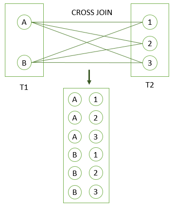
CROSS JOIN

A CROSS JOIN clause allows you to produce a Cartesian Product of rows in two or more tables.

Different from other join clauses such as LEFT JOIN or INNER JOIN, the CROSS JOIN clause does not have a join predicate.

Suppose you have to perform a CROSS JOIN of two tables T1 and T2. If T1 has n rows and T2 has m rows, the result set will have nxm rows.

1
2
3

SELECT select_list
FROM T1
CROSS JOIN T2;

self-join

A self-join is a regular join that joins a table to itself. In practice, you typically use a self-join to query hierarchical data or to compare rows within the same table.

1
2
3
4
5
6
7

SELECT
    e.first_name || ' ' || e.last_name employee,
    m .first_name || ' ' || m .last_name manager
FROM
    employee e
INNER JOIN employee m ON m .employee_id = e.manager_id
ORDER BY manager;

USING Clause

The USING clause specifies which columns to test for equality when two tables are joined. It can be used instead of an ON clause in the JOIN operations that have an explicit join clause.

The following query performs an inner join between the countries table and the cities table on the condition that countries.countryis equal to cities.country:

1

SELECT * FROM countries JOIN cities USING (country);

The next query is similar to the one above, but it has the additional join condition that countries.countryis equal to cities.country_iso_code:

1

SELECT * FROM countries JOIN cities USING (country, country_iso_code);

SELECT … INTO Statement

GROUP BY Clause

The GROUP BY clause divides the rows returned from the SELECT statement into groups. For each group, you can apply an aggregate function e.g., SUM() to calculate the sum of items or COUNT() to get the number of items in the groups.

 1
 2
 3
 4
 5
 6
 7
 8
 9
10
11

SELECT 
   column_1, 
   column_2,
   ...,
   aggregate_function(column_3)
FROM 
   table_name
GROUP BY 
   column_1,
   column_2,
   ...;

1. Using GROUP BY without an aggregate function

   1 2 3 4 5 6

   SELECT customer_id FROM payment GROUP BY customer_id;

2. Using GROUP BY with SUM() function

   1 2 3 4 5 6 7

   SELECT customer_id, SUM (amount) FROM payment GROUP BY customer_id;

3. Using GROUP BY clause with the JOIN clause

   1 2 3 4 5 6 7 8 9

   SELECT first_name || ' ' || last_name full_name, SUM (amount) amount FROM payment INNER JOIN customer USING (customer_id) GROUP BY full_name ORDER BY amount DESC;

4. Using GROUP BY with COUNT() function

   1 2 3 4 5 6 7

   SELECT staff_id, COUNT (payment_id) FROM payment GROUP BY staff_id;

5. Using GROUP BY with multiple columns

   1 2 3 4 5 6 7 8 9 10 11

   SELECT customer_id, staff_id, SUM(amount) FROM payment GROUP BY staff_id, customer_id ORDER BY customer_id;

6. Using GROUP BY clause with a date column

   1 2 3 4 5 6 7

   SELECT DATE(payment_date) paid_date, SUM(amount) sum FROM payment GROUP BY DATE(payment_date);

HAVING Clause

The HAVING clause specifies a search condition for a group or an aggregate. The HAVING clause is often used with the GROUP BY clause to filter groups or aggregates based on a specified condition.

The HAVING clause, like the WHERE clause, specifies selection conditions. The WHERE clause specifies conditions on columns in the select list, but cannot refer to aggregate functions. The HAVING clause specifies conditions on groups, typically formed by the GROUP BY clause. The query result includes only groups satisfying the HAVING conditions. (If no GROUP BY is present, all rows implicitly form a single aggregate group.)

1
2
3
4
5
6
7
8
9

SELECT
	customer_id,
	SUM (amount)
FROM
	payment
GROUP BY
	customer_id
HAVING
	SUM (amount) > 200;

1
2
3
4
5
6
7
8
9

SELECT
	store_id,
	COUNT (customer_id)
FROM
	customer
GROUP BY
	store_id
HAVING
	COUNT (customer_id) > 300;

Confirming Indexes

It will show you all the indexes present in the server.

1

SELECT * from USER_INDEXES;

Aliases

Column Aliases

1

SELECT column as alias_name FROM table_name;

Standard SQL disallows references to column aliases in a WHERE clause. This restriction is imposed because when the WHERE clause is evaluated, the column value may not yet have been determined.

In the select list of a query, a quoted column alias can be specified using identifier or string quoting characters:

1

SELECT 1 AS `one`, 2 AS 'two';

Elsewhere in the statement, quoted references to the alias must use identifier quoting or the reference is treated as a string literal.

Table Alias

1

SELECT column FROM table_name as alias_name;

Subqueries

The Subquery as Scalar Operand Comparisons Using Subqueries

Subqueries with ANY, IN, or SOME

ANY compares a value to each value in a list or results from a query and evaluates to true if the result of an inner query contains at least one row.

1
2
3

operand comparison_operator ANY (subquery)
operand IN (subquery)
operand comparison_operator SOME (subquery)

Where comparison_operator is one of these operators:

1

=  >  <  >=  <=  <>  !=

When used with a subquery, the word IN is an alias for = ANY. IN and = ANY are not synonyms when used with an expression list. IN can take an expression list, but = ANY cannot.

The word SOME is an alias for ANY.

Subqueries with ALL

The ALL operator returns TRUE if all of the subqueries values meet the condition

1

operand comparison_operator ALL (subquery)

In general, tables containing NULL values and empty tables are “edge cases.” When writing subqueries, always consider whether you have taken those two possibilities into account.

NOT IN is an alias for <> ALL.

Subqueries with EXISTS

The EXISTS condition in SQL is used to check whether the result of a correlated nested query is empty (contains no tuples) or not. The result of EXISTS is a boolean value True or False.

1
2
3
4
5
6
7

SELECT 
	fname, lname 
FROM 
	customers 
WHERE EXISTS (SELECT * 
              FROM orders 
              WHERE customers.id = orders.customer_id);

Row Subqueries Subqueries with EXISTS or NOT EXISTS Correlated Subqueries Derived Tables Lateral Derived Tables Subquery Errors Optimizing Subqueries Restrictions on Subqueries

Data manipulation language (DML)

INSERT Statement

The first method is to specify only the value of data to be inserted without the column names.

1

INSERT INTO table_name VALUES (value1, value2, value3); 

In the second method we will specify both the columns which we want to fill and their corresponding values.

1

INSERT INTO table_name (column1, column2, column3) VALUES (value1, value2, value3); 

INSERT IGNORE Statement

This means that an INSERT IGNORE statement which contains a duplicate value in a UNIQUE index or PRIMARY KEY field does not produce an error, but will instead simply ignore that particular INSERT command entirely.

1

INSERT IGNORE INTO table_name (column1, column2, column3) VALUES (value1, value2, value3); 

INSERT … SELECT Statement

We can use the SELECT statement with INSERT INTO statement to copy rows from one table and insert them into another table.

1

INSERT INTO first_table(col_name1, col_name2) SELECT col_name1, col_name2 FROM second_table WHERE condition;

INSERT … ON DUPLICATE KEY UPDATE Statement INSERT DELAYED Statement

UPDATE Statement

1

UPDATE table_name SET column1 = value1, column2 = value2,… WHERE condition;

DELETE Statement

Deleting a row from a view first delete the row from the actual table and the change is then reflected in the view.

1

DELETE FROM table_name WHERE condition;

MERGE Statement

1
2
3
4
5
6
7
8
9

MERGE target_table_name AS target_alias
USING source_table_name AS source_alias  
ON join_condition
WHEN MATCHED THEN
	UPDATE ...
WHEN NOT MATCHED BY TARGET THEN
	INSERT ...
WHEN NOT MATCHED BY SOURCE THEN 
	DELETE ...

1
2
3
4
5
6
7
8

MERGE INTO customer_account ca
USING recent_transactions t
ON t.customer_id = ca.customer_id
WHEN MATCHED THEN
  UPDATE SET balance = balance + transaction_value
WHEN NOT MATCHED THEN
  INSERT (customer_id, balance)
  VALUES (t.customer_id, t.transaction_value);

UNION Clause

UNION combines the result from multiple query blocks into a single result set.

If neither DISTINCT nor ALL is specified, the default is DISTINCT. DISTINCT can remove duplicates from either side of the intersection.

The operands must have the same number of columns.

1

query1 UNION [ALL] query2

INTERSECT Clause

INTERSECT limits the result from multiple query blocks to those rows which are common to all.

If neither DISTINCT nor ALL is specified, the default is DISTINCT. DISTINCT can remove duplicates from either side of the intersection.

The operands must have the same number of columns.

1

query1 INTERSECT [ALL] query2

INTERSECT has greater precedence than and is evaluated before UNION and EXCEPT, so that the two statements shown here are equivalent:

1
2
3

TABLE r EXCEPT TABLE s INTERSECT TABLE t;

TABLE r EXCEPT (TABLE s INTERSECT TABLE t);

EXCEPT Clause

EXCEPT limits the result from the first query block to those rows which are (also) not found in the second.

If neither DISTINCT nor ALL is specified, the default is DISTINCT. DISTINCT can remove duplicates from either side of the intersection.

The operands must have the same number of columns.

1

query1 EXCEPT [ALL] query2

Difference between EXCEPT and NOT IN Clause: EXCEPT automatically removes all duplicates in the final result, whereas NOT IN retains duplicate tuples. It is also important to note that EXCEPT is not supported by MySQL.

CALL Statement

Call a PL/SQL or JAVA subprogram.

LOCK Statement

Table control concurrency.

EXPLAIN PLAN Statement

It describes the access path to data.

DO Statement EXCEPT Clause HANDLER Statement

INTERSECT Clause LOAD DATA Statement LOAD XML Statement Parenthesized Query Expressions REPLACE Statement

Set Operations with UNION, INTERSECT, and EXCEPT

TABLE Statement

UNION Clause VALUES Statement

IMPORT TABLE Statement

WITH (Common Table Expressions)

A common table expression (CTE) is a named temporary result set that exists within the scope of a single statement and that can be referred to later within that statement, possibly multiple times.

The following example defines CTEs named cte1 and cte2 in the WITH clause, and refers to them in the top-level SELECT that follows the WITH clause:

1
2
3
4
5

WITH
  cte1 AS (SELECT a, b FROM table1),
  cte2 AS (SELECT c, d FROM table2)
SELECT b, d FROM cte1 JOIN cte2
WHERE cte1.a = cte2.c;

In the statement containing the WITH clause, each CTE name can be referenced to access the corresponding CTE result set.

Data control language (DCL)

GRANT Statement

1

GRANT create table, create view TO role_name;

1

GRANT role_name TO user1, user2;

1

Grant SELECT,INSERT,UPDATE,DELETE on table_name To user_or_role

REVOKE Statement

1

REVOKE create table FROM role_name;

1

Revoke INSERT On table_name FROM user_or_role

Transaction control language (TCL)

A database transaction, by definition, must be atomic, consistent, isolated, and durable.

These are popularly known as ACID properties. These properties can ensure the concurrent execution of multiple transactions without conflict.

Properties of Transaction:

• Atomicity: The outcome of a transaction can either be completely successful or completely unsuccessful. The whole transaction must be rolled back if one part of it fails.
• Consistency: Transactions maintain integrity restrictions by moving the database from one valid state to another.
• Isolation: Concurrent transactions are isolated from one another, assuring the accuracy of the data.
• Durability: Once a transaction is committed, its modifications remain in effect even in the event of a system failure.

BEGIN Statement

Start a new transaction.

1

BEGIN TRANSACTION transaction_name;

SET Statement

The values for the properties of the current transaction, such as the transaction isolation level and access mode.

1

SET TRANSACTION [ READ WRITE | READ ONLY ];

COMMIT Statement

Commits a Transaction.

The COMMIT command saves all the transactions to the database since the last COMMIT or ROLLBACK command.

1

COMMIT;

ROLLBACK Statement

Rollbacks a transaction in case of any error occurs. This command can only be used to undo transactions since the last COMMIT or ROLLBACK command was issued.

1

ROLLBACK;  

SAVEPOINT Statement

Sets a save point within a transaction.

SAVEPOINT creates points within the groups of transactions in which to ROLLBACK.

A SAVEPOINT is a point in a transaction in which you can roll the transaction back to a certain point without rolling back the entire transaction.

1

SAVEPOINT savepoint_name;

Syntax for rolling back to Savepoint Command:

1

ROLLBACK TO savepoint_name;

RELEASE Statement

This command is used to remove a SAVEPOINT that you have created.

1

RELEASE SAVEPOINT savepoint_name

START TRANSACTION, COMMIT, and ROLLBACK Statements

START TRANSACTION, COMMIT, and ROLLBACK Statements Statements That Cannot Be Rolled Back Statements That Cause an Implicit Commit SAVEPOINT, ROLLBACK TO SAVEPOINT, and RELEASE SAVEPOINT Statements LOCK INSTANCE FOR BACKUP and UNLOCK INSTANCE Statements LOCK TABLES and UNLOCK TABLES Statements SET TRANSACTION Statement XA Transactions

Compound Statement Syntax

Flow Control Statements

CASE Statement

1
2
3
4
5

CASE case_value
    WHEN when_value THEN statement_list
    [WHEN when_value THEN statement_list] ...
    [ELSE statement_list]
END CASE

Or:

1
2
3
4
5

CASE
    WHEN search_condition THEN statement_list
    [WHEN search_condition THEN statement_list] ...
    [ELSE statement_list]
END CASE

Utility Statements

DESCRIBE Statement

1

DESCRIBE table_name;

Reference

SQL Tutorial

SQL Tutorial

Learn SQL

Intro to SQL

SQL in 10 Minutes, Sams Teach Yourself

SQL必知必会

SQLBolt